Automate surface threat evaluation on naval vessels with limited capabilities

Abstract

Finding an efficient threat evaluation computational model for warships is usually a complex task with limited study in general, however, the task can be even more complicated when conceiving a model for naval vessels with limited capacity such as ocean or coastal patrol vessels, which in many cases only have a single two-dimensional surveillance radar for surface contacts. The purpose of this study is to develop a computational model that satisfies this problem by reviewing the state of the art in the development of these technologies, comparing models and algorithms used in previous works, using as input source information of a 2D surveillance radar and analyzing the kinetic information detected from other contacts present in the environment, comparing different types of implementation and finding through the evaluation of the results obtained, the most accurate conclusions that allow integrating this model to a military decision support system of national development in the near future.

Video

Radar 2D view simulation with Surface Threat Evaluation algorithm

Method

Next, we will detail the design and development process of the solution implemented within the framework of this study which evaluated the algorithms and methods used so far to solve the Threat Evaluation problem for surface platforms in conventional and non-conventional warfare scenarios, based on Bayesian Network and Fuzzy Logic approachs. The following is a graphical simplification of the designed model.

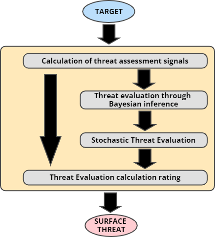
Calculation of threat assessment signals

Implementing a computational model that satisfies the operational needs in the evaluation and classification of threats for a maritime environment, from the perspective of naval tactics, tends to become a costly task due to the complexity involved in trying to parameterize specific situations in unique and general algorithms, which in the eyes of official experts on the subject can be confusing when transferring the problem to a field of computing. However, understanding that this type of solutions are never intended to replace human judgment and expertise, but on the contrary, they are intended to facilitate the command and control process by generating Decision Support Systems (DSS) that can optimize the appropriate decision making in a naval context. The evaluation of variables necessary to build this type of models, consider the object of this study must take into account the analysis of data related to the movement acquired by radar, but the parameterization of which data are relevant or not in the inference of threat, as well as determining the proportion between the chosen variables must take into account the information provided by experts in the subject.

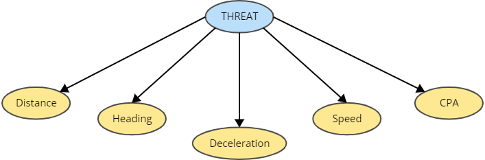
The cues considered for this study, like in the study of Çöçelli & Arkin are Distance, Heading, Deceleration, Speed, Closest Point of Approach (CPA), and TBH (Time Before Hit). But with few variants in some of these cues as detailed as follows:

Distance

The distance is the evidence considered as the distance within a two-dimensional plane on the surface of the earth between the secured asset (own ship), and the radar contact to be evaluated as a possible threat. This distance can be considered as the distance obtained through the haversine formula to compute the distance between objects in the plane of an ellipsoid modeled on the surface of the earth, these calculations are based on geographic and geospatial referencing with reference to the World Geodetic System of 1984 (WGS-84). This evidence can be considered as the most relevant within the motion data obtained by a conventional radar taking into account the conclusions of different studies conducted by the US Navy related in (Liebhaber D A Kobus & Feher SSC San Diego, 2002), as well as in (Liebhaber & Feher, 2002b). For this purpose, the following formula proposed by Çöçelli & Arkin is used to calculate the evidence given by:

Where represents the final value of the evidence to be calculated, represents the actual measured value of the distance between the contact to be evaluated and the vessel itself, and represents the maximum value of distance to be considered.

For this cue, the maximum distance considered in the formula, are the calculous of radar horizon given by the expression:

Where represents the maximum distance from the radar horizon, represents the earth radius datum given by =6.371,01 Km, and represents the height of the radar antenna on the mast of the parameterized surface vessel.

Heading

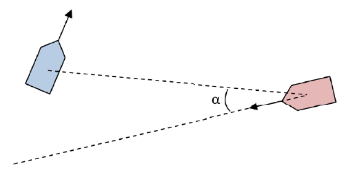
Heading is important evidence, which is fundamental to infer the intentionality of a surface contact on my own vessel, since, if it demonstrates with its heading a direct direction towards the defended asset, it can be considered as an indicator of great relevance in terms of threat evaluation. On the contrary, if the heading of the contact is not related to a direction towards the defended asset, it can be considered in terms of intentionality as a factor of little interest or representing some kind of threat to my own vessel. The value of this evidence is calculated considering the relationship between the projection of the true heading vector of the contact, and the azimuth by which this contact is detected. The angle formed by the intersection of the two vectors may point to some measure of interest to perform an inference calculation regarding its threat level. For this purpose, the following formula proposed by Çöçelli & Arkin is used to calculate the evidence given by:

Where represents the final value of the evidence to be calculated, represents the value of the angle calculated between the intersection of the projection of the contact bearing and the true bearing of which it is detected, and represents the value of the maximum angle expressed in radians to be considered.

The bellow calculation consider in this study the time of the CPA (Closest Point of Approach), if this value is positive, two different conditions are evaluated, if the defeated asset (own ship) is quite, the max angle is considered by , otherwise, the max angle evaluated will be . In case the value of the time of CPA were negative, the cue value will be set to zero.

For the calculation of the variable is to consider the following figure where the blue figure represents the insured asset (own ship), and the red figure represents the contact object of inference. This is for the purpose of visually clarifying the concept of the cue:

Deceleration

The evidence is considered as evidence that adds value to the inference of threat on a specific contact, this statement is based on studies by Liebhaber & Feher, where the value of change of threat rating for surface contacts is highly influenced by the decrease of detected velocity of a surface contact. This indicator of intentionality can infer certain threat since it is an indicator of readiness for possible hostile actions, likewise the fact that a surface contact in a specific sea lane decreases its speed is an abnormal indicator of its expected behavior. For this purpose, the following formula proposed by Çöçelli & Arkin is used to calculate the evidence given by:

Where represents the final value of the evidence to be calculated, represents the current value of the speed detected by radar, represents the previous value of the speed detected for the same radar contact, and represents the maximum value of the speed to be considered.

Speed

Speed is one of the most considered indicators of intentionality in the inference of hostility on a contact, this evidence is a fundamental part of the calculation of variables to generate a fairly close approximation of probability of threat or not on a surface contact, however it is not considered as one of the most relevant factors in terms of classification of the most influential variables on the evaluation of threats according to the studies of Liebhaber & Feher. For this purpose, the following formula proposed by Çöçelli & Arkin is used to calculate the evidence given by:

Where represents the final value of the evidence to be calculated, represents the actual value of the speed detected by radar, and represents the maximum value of the speed to be considered.

Closest Point of Approach (CPA)

Is one of the best-known types of evidence within the maritime industry for threat evaluation, it is widely known in civilian and military environments and is even applicable to aerial environments. The maximum value used in the formula proposed by Çöçelli & Arkin, are defined by the most common range gun-nery, most warships carry smaller guns, with the 76 mm (3 inch) gun being very common throughout the world according J. L. George.

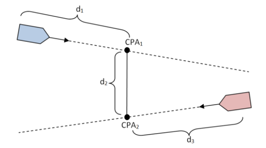
The calculation of this variable refers to the calculation of the trajectory projection of a contact in order to determine the minimum distance at which this contact will perform a close distance relation over the defended asset (own ship), over transit on its same trajectory.

For this purpose, the following formula proposed by Çöçelli & Arkin is used to calculate the evidence given by:

Where represents the final value of the evidence to be calculated, represents the current calculated value of the CPA according to the data obtained by radar, and represents the maximum value of the CPA to be considered.

Time Before Hit (TBH)

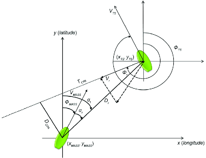
This evidence is of great interest on the intentionality of a contact since it is related to the calculated time in which the contact will follow a collision trajectory towards the own ship taking as reference a trajectory based on the Closest Point of Approach. For illustrative purposes, the graphic concept of its meaning is shown below:

For this purpose, the following formula proposed by Çöçelli & Arkin is used to calculate the evidence given by:

Given,

Where represents the final value of the evidence to be calculated, represents the current calculated value of the TBH, represents the maximum value of the TBH to be considered and represents the value of the current velocity recorded by the contact.

However, for this study a conditionality factor given by the calculation of the Time of Closest Point of Approach (TCPA) has to be considered, considering that a negative time variable symbolizes a past event and does not represent an indicator of relevance for the computation of this particular evidence, the calculation of this variable was detailed in the description of the evidence of the Closest Point of Approach (CPA).

Time to Closest Point of Approach (TCPA)

For this study, it represents conditional evidence not evaluated directly in the Bayesian network by reason of conditional independence necessary in a Bayesian Network, but will be fundamental to determine some conditional rules in cues calculation like CPA, Heading and TBH.

Threat Evaluation through Bayesian inference

Bayes’ theorem provides a simple method for calculating the probability of an event given some evidence. Representing the threat hypothesis for a contact, it represents itself a Boolean value (threat, non-threat) represented by mutually exhaustive and exclusive states according to general probability concepts, the formulas is considered as:

However, if represents the threat hypothesis for a contact, it represents itself a Boolean value (threat, non-threat) represented by mutually exhaustive and exclusive states according to general probability concepts. Therefore, the general Bayes theorem previously defined is redefined according to the following formula:

Bayesian network graphical model definition

In this particular case, having previously the variables defined by the model of Çöçelli & Arkın, 2017 it is known that the set of variables and their level of granularity are given by the evidences of Distance, Heading, Deceleration, Speed and PMA previously defined, where it was specified that the evidence of TBH is not considered for the modeling of the Bayesian network given its incompatibility of conditional independence as it is dependent on the evidence of speed. Therefore, it is possible to model the directed acyclic graph of a Bayesian network as follows:

Under the structure of the above ilustration, it is possible to classify the type of network as Divergent Connection (common cause), or also known as Naïve Bayes Classifier. On this pretext, the identified evidences (clues) are conditionally independent given the parent node (threat), which is also equivalent to say that the given evidences are d-separated by the threat. Therefore, the evidence can be transmitted between the indicia through the divergent connection of the threat, unless the threat is instantiated. Therefore, given the Bayesian network formulation considerations proposed by the above model, we reformulate the Bayes theorem for the exact inference calculation given by the following statement:

Where,

The expressions are given by the multiplication rule for dependent events.

The expression represents the total probability given the parameterization of the modeled Bayesian network.

The expression represents the a posteriori conditional probability of (Threat), given (logical conjunction of the 5 evidences).

The expression represents the a priori conditional probability of (logical conjunction of the 5 evidences), given (A priori Threat).

The expression represents the a priori conditional probability of (logical conjunction of the 5 evidences), given (No a priori Threat).

The expression represents the marginal a posteriori probability of (Threat).

The expression represents the a priori marginal probability of (Threat).

The expression represents the a priori marginal probability of (No Threat).

It should be noted that according to the previously reformulated theorem, within the framework of the present study, the a priori term refers to the probabilities determined by the conditional probability tables (CPT), and the a posteriori term refers to the calculation of the resulting Bayesian inference.

Stochastic Threat Evaluation

When evaluating the model as a function of time, it should be noted that threat evaluation through Bayesian inference is framed in a stochastic process since radar information allows the update of data on a specific target that can be used to update the probability inference. The use of dynamic Bayesian inference represents the evolution of some state space time model over time, in which objects change state dynamically. For the case of the model proposed in this study, an additional novel method is proposed within the process of threat inference on a surface target with multiple time varying states by updating data from the radar simulator. For this purpose, use is made of the result of Bayesian inference in a previous state, which updates the marginal probability of threat, being this new marginal probability the one used for a Bayesian inference process later. The stochastic evaluation proposed in this study is only considered to the targets detected out of closest distance state in the layered distance CPT (Conditional Probability Table). The marginal probability considered in the closest distance state will have a raised fixed value (non stochastic), considering the distance as the most important cue for threat inference according to the studies developed by the U.S. Navy.

Threat Evaluation calculation rating

The final step is generating a prioritized list of targets classified as threat, this study follows the guidelines proposed in the study of Çöçelli & Arkin. The importance of each cue is determined by the importance of the cue determined by M. J. Liebhaber. In this part of the algorithm, the TBH cue is evaluated only since the Bayes-ian Network don’t allow it to avoid conditional independence issues in the model. For the formulation of this phase, each piece of evidence is computed by the weight it represents for the prioritization of signals as the follow expression:

Where represents the weight coefficient for each piece of evidence within the general model, therefore, the model is formulated by the following expression:

Given,

And,

Where,

Where represents the total ranking calculation for the threat assessment represented by the contribution of each evidence, given by the summation of the calculation of each evidence and its respective coefficient. are the overall threat values within a tactical scenario evaluated with different surface targets considered (according to situational awareness), and therefore represents the contribution of each evidence considered in the model.

Therefore, in general, the contribution of each piece of evidence considered in this step of the algorithm can be modeled explicitly by reformulating in the following expression in terms of the contribution of each piece of evidence:

being the overall calculation of the hazard assessment rating for each target, given by as the coefficient of each evidence, the contribution of the distance evidence, the contribution of the heading evidence, the contribution of the deceleration evidence, the contribution of the velocity evidence, and the contribution of the TBH evidence.

Evaluation

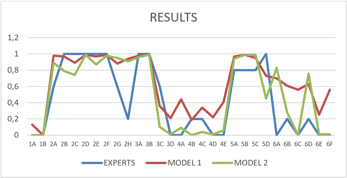
The process to evaluate the behavior in the proposed model considered the use of a 2D radar simulator to characterize scenarios measuring target performance to a defended asset, those scenarios were contrasted through expert opinion from the Colombian Navy comparing inference results for each scenario. The results from each kinetic patron were compared between experts opinions and the model threat inference trough the Brier Score method to measure the score in the proposed model to compare it accuracy, where the closer the Brier Score is to zero, the better the prediction is. Six scenarios were organized considering the experience of the author of this study as a surface officer, from least to most difficult, from the “easiest” to infer, to the “hardest” to infer, and taking as input the feedback from the respondents considered. The contrasted data consider the model proposed by Çöçelli & Arkin as model 1, and the model proposed in this study as model 2. The results from all scenarios in each stage are displayed in the next graphic:

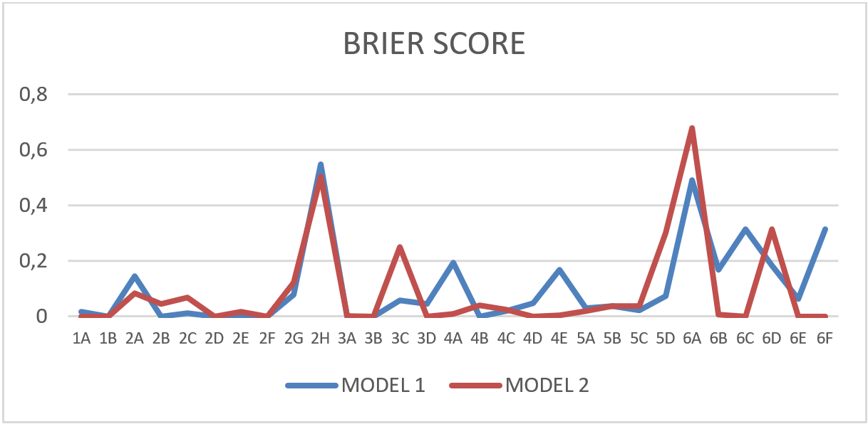
Contrasting the data with the Brier Score method, considering the lowest score (near to zero) is more accurate, the following graphic show the results processed from the above Figure:

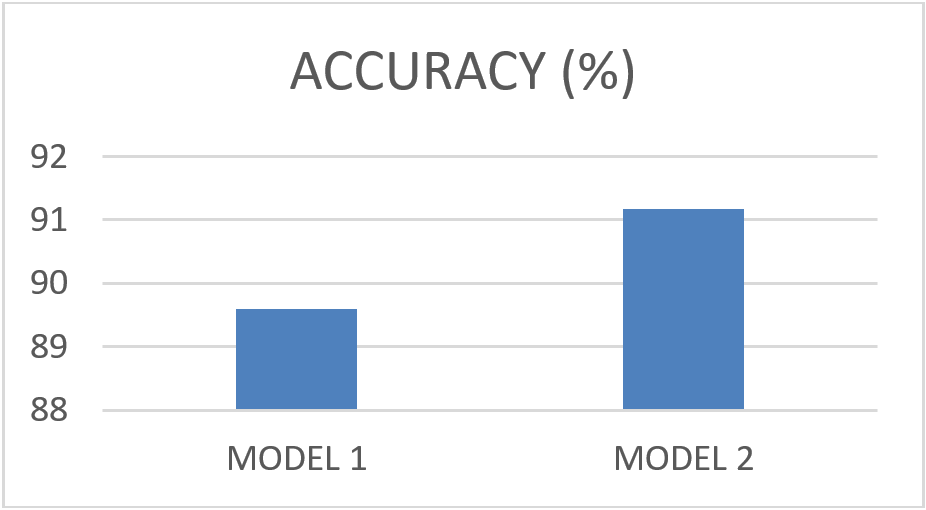
The average data from Brier Score obtained in above Figure, could be expressed in term of the accuracy of each model represented by the following graphic:

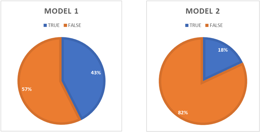
Considering the whole events (targets) detected by each scenario, the quantity of threats classified by each model give an extra information related to the reliability of each one considering the general purpose to this kind of systems is to be a Decision Support System. The following data compares the quantity of classified threats by each one:

SCENARIOS	MODEL	1	MODEL	2
SCENARIOS	TRUE	FALSE	TRUE	FALSE
Scenario 1	368	486	184	670
Scenario 2	330	343	131	542
Scenario 3	378	621	187	812
Scenario 4	213	317	29	501
Scenario 5	230	283	112	401
TOTAL	1519	2050	643	2926
PROPORTION	42.56%	57.43%	18.01%	81.98%

Conclusions

As the result of this study, the different techniques and algorithmic approaches used for threat evaluation were identified through the study of the art, and the best related technique for limited information from available sensors, such as a 2D surface radar in naval units with limited capabilities, according to the study of Çöçelli & Arkın.

The model comparison presented in this study, was able to contrast through the results, that model No. 2 (stochastic evaluation of the author) has the highest level of accuracy to the result of the representative value of the respondents in comparison to model No. 1. Likewise, it was determined in the comparison of the models that the proposals developed by the author, represent more congruent data for a Decision Support System (DSS) in the classification of threats, since almost half of the events in model No. 1 are classified as a threat.

References

1. F. Johansson, Evaluating the Performance of TEWA Systems, Skövde, Sweden: örebro university, 2010.
2. N. Šerbedžija, “Simulating Artificial Neural Networks on Parallel Architectures,” Institute of Electrical and Electronics Engineers, p. 8, 1996.
3. A. X. Dong and L. G. Qing, “Application of Neural Networks in the Field of Target Threat Evaluation,” Institute of Electrical and Electronics Engineers, p. 4, 1999.
4. G. Blasco Jimenez, “Modelos gráficos probabilísticos en sistemas distribuidos,” Universitat de Barcelona, Barcelona, 2015.
5. A. Benavoli, B. Ristic, A. Farina, M. Oxenham and L. Chisci, “An Approach to Threat Assessment Based on Evidential Networks,” Institute of Electrical and Electronics Engineers, p. 8, 2007.
6. N. Fenton and M. Neil, Risk assessment and decision analysis with Bayesian networks, Boca Ratón: CRC Press, 2019.
7. N. Okello and G. Thoms, “Threat Assessment Using Bayesian Networks,” in Proceedings of the Sixth International Conference of Information Fusion, 2003., Cairns, QLD, Australia, 2003.
8. M. Çöçelli and E. Arkın, “A Category Based Threat Evaluation Model Using Platform Kinematics Data,” Advances in Science, Technology and Engineering Systems Journal, vol. 2, no. 3, pp. 1330-1341, 2017.
9. M. J. Liebhaber and C. A. Smith, “Naval Air Defense Threat Assessment: Cognitive Factors and Model,” Space and Naval Warfare Systems Center,, San Diego, CA, 2000.
10. M. J. Liebhaber, “Surface Warfare Threat Assesment: Requirement Definition,” SPAWAR System Center San Diego, 2002, 2002.
11. CMCON, «Dinámica del Narcotráfico Marítimo» Informe CMCON, vol. 004, p. 112, 2020.
12. J. L. George, History of warships: From ancient times to the twenty-first century, Annapolis, MD.: Naval Institute Press, 1998.

---

---

Hosted on GitHub Pages - Theme by orderedlist